workshops
Error Bars and Misconceptions
Misconceptions
-
Misinterpretation of Error Bars: Error bars are frequently misunderstood in terms of what they signify about statistical significance, particularly when comparing the overlap of error bars from different data sets.
-
Confusing SD with SEM: There is often a mix-up between standard deviation (SD) and standard error of the mean (SEM). SD error bars tell about the variability within the population, whereas SEM bars inform about the uncertainty of the estimated mean, which is influenced by sample size.
-
Misconception about Confidence Intervals: A common error is the belief that a 95% confidence interval (CI) indicates that there is a 95% probability that the interval contains the true population mean, which is a misinterpretation of how confidence intervals function statistically.
library(tidyverse)

set.seed(123)
ratings <- tibble(rating = rnorm(100, mean = 3, sd = 0.5))

stats <- summarise(ratings,
                   mean_rating = mean(rating),
                   sd_rating = sd(rating),
                   se_rating = sd_rating / sqrt(n()),
                   ci80 = qnorm(1 - 0.10/2) * se_rating,
                   ci95 = qnorm(1 - 0.05/2) * se_rating,
                   ci99 = qnorm(1 - 0.01/2) * se_rating)

data <- tibble(
  x = rep(1, 100),
  y = ratings$rating,
  ymin = NA_real_,
  ymax = NA_real_,
  group = "Jitter"
)

stats_data <- tibble(
  x = 2:6,
  y = rep(stats$mean_rating, 5),
  ymin = stats$mean_rating - c(stats$sd_rating, stats$se_rating, stats$ci80, stats$ci95, stats$ci99),
  ymax = stats$mean_rating + c(stats$sd_rating, stats$se_rating, stats$ci80, stats$ci95, stats$ci99),
  group = c("SD", "SE", "CI80", "CI95", "CI99")
)

data <- bind_rows(data, stats_data)
head(data)
| x | y | ymin | ymax | group |
|---|---|---|---|---|
| <dbl> | <dbl> | <dbl> | <dbl> | <chr> |
| 1 | 2.719762 | NA | NA | Jitter |
| 1 | 2.884911 | NA | NA | Jitter |
| 1 | 3.779354 | NA | NA | Jitter |
| 1 | 3.035254 | NA | NA | Jitter |
| 1 | 3.064644 | NA | NA | Jitter |
| 1 | 3.857532 | NA | NA | Jitter |
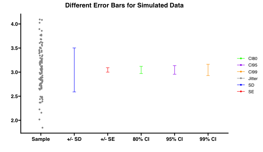
colors <- c("Jitter" = "grey60", "SD" = "blue", "SE" = "red", "CI80" = "green", "CI95" = "purple", "CI99" = "orange")

p <- ggplot(data, aes(x = as.factor(x), y = y, ymin = ymin, ymax = ymax, color = group)) +
  geom_jitter(data = filter(data, group == "Jitter"), width = 0.05) +
  geom_errorbar(data = filter(data, group != "Jitter"), width = 0.1, position = position_dodge(width = 0.8)) +
  scale_color_manual(values = colors) +
  scale_x_discrete(labels = c("Sample", "+/- SD", "+/- SE", "80% CI", "95% CI", "99% CI")) +
  labs(title = "Different Error Bars for Simulated Data", x = "Simulated Data", y = "") +
  theme(axis.title.x = element_blank(), axis.text.x = element_text(angle = 45, hjust = 1), legend.title = element_blank())

print(p)
library(ggplot2)
mean1 <- 5
mean2 <- 4
n <- 10
alpha <- 0.05
t_critical <- qt(1 - alpha/2, df=(n-1)*2)
std_dev_estimated <- abs(mean1 - mean2) / t_critical * sqrt(n/2)
sem1 <- std_dev_estimated / sqrt(n)
sem2 <- std_dev_estimated / sqrt(n)
ci_half_width1 <- t_critical * sem1
ci_half_width2 <- t_critical * sem2
data <- data.frame(
type = rep(c('STD', 'SEM', 'CI'), each = 2),
sample = factor(rep(c('Sample 1', 'Sample 2'), 3)),
mean = c(mean1, mean2, mean1, mean2, mean1, mean2),
ymin = c(mean1 - std_dev_estimated, mean2 - std_dev_estimated,
mean1 - sem1, mean2 - sem2,
mean1 - ci_half_width1, mean2 - ci_half_width2),
ymax = c(mean1 + std_dev_estimated, mean2 + std_dev_estimated,
mean1 + sem1, mean2 + sem2,
mean1 + ci_half_width1, mean2 + ci_half_width2)
)
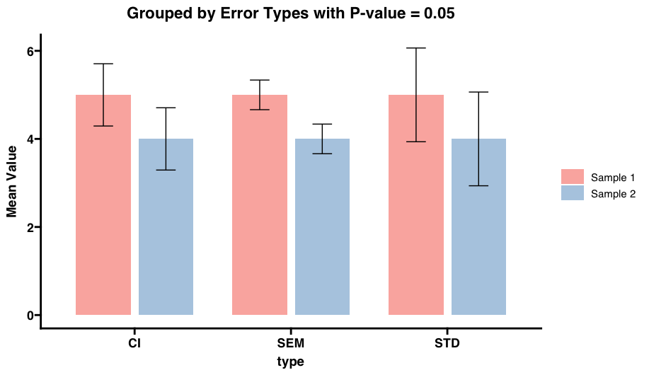
p <- ggplot(data, aes(x = type, y = mean, fill = sample)) +
geom_bar(stat = "identity", position = position_dodge(width = 0.8), width = 0.7) +
geom_errorbar(aes(ymin = ymin, ymax = ymax), position = position_dodge(width = 0.8), width = 0.25) +
theme_minimal() +
labs(title = "Grouped by Error Types with P-value = 0.05", y = "Mean Value") +
scale_fill_brewer(palette = "Pastel1", name = "Sample")
print(p)
Guidance on Using Standard Deviation, Standard Error, and Confidence Intervals as Errors When Plotting Data
- Standard Deviation (SD):
- Use SD to represent the variability or dispersion of a set of data points around the mean.
- SD is most appropriate when you want to show how much individual measurements in a dataset vary from the average value.
- Ideal for datasets where you’re interested in the distribution of values itself, rather than estimating the reliability of a sample mean.
- Standard Error (SE):
- Use SE to represent the precision of the sample mean as an estimate of the population mean.
- SE is calculated as the standard deviation of the sample divided by the square root of the sample size.
- Appropriate for datasets where the goal is to infer about the population from a sample, especially in cases where multiple samples are compared.
- Confidence Intervals (CI):
- Use CIs to provide a range within which the true population parameter is expected to lie, with a certain level of confidence (usually 95% or 99%).
- CI gives an estimated range of values which is likely to include the population parameter, based on the sample data.
- Ideal for both visualizing the precision of sample estimates and making inferences about the population, particularly useful in comparative studies.
Important Points:
- SD emphasizes the variability or spread of the data.
- SE provides a measure of the accuracy of the sample mean.
- CI offers an estimated range that is likely to include the population parameter, indicating the reliability of an estimate.
Considerations:
- When plotting data with errors, your choice among SD, SE, and CI should align with the story you want the data to tell. Are you focusing on the spread of the data, the precision of the sample mean, or the range within which the population mean likely falls?
- The use of SE and CI is particularly relevant in hypothesis testing and when the sample size is relatively small compared to the population.
- Always specify what measure of error you are using in your plots to avoid misinterpretation.
Reference
- Krzywinski, M., & Altman, N. (2013). Error bars. Nature Methods, 10(10), 921-922. https://doi.org/10.1038/nmeth.2659