workshops
Last Updated: 2024-10-03
RStudio
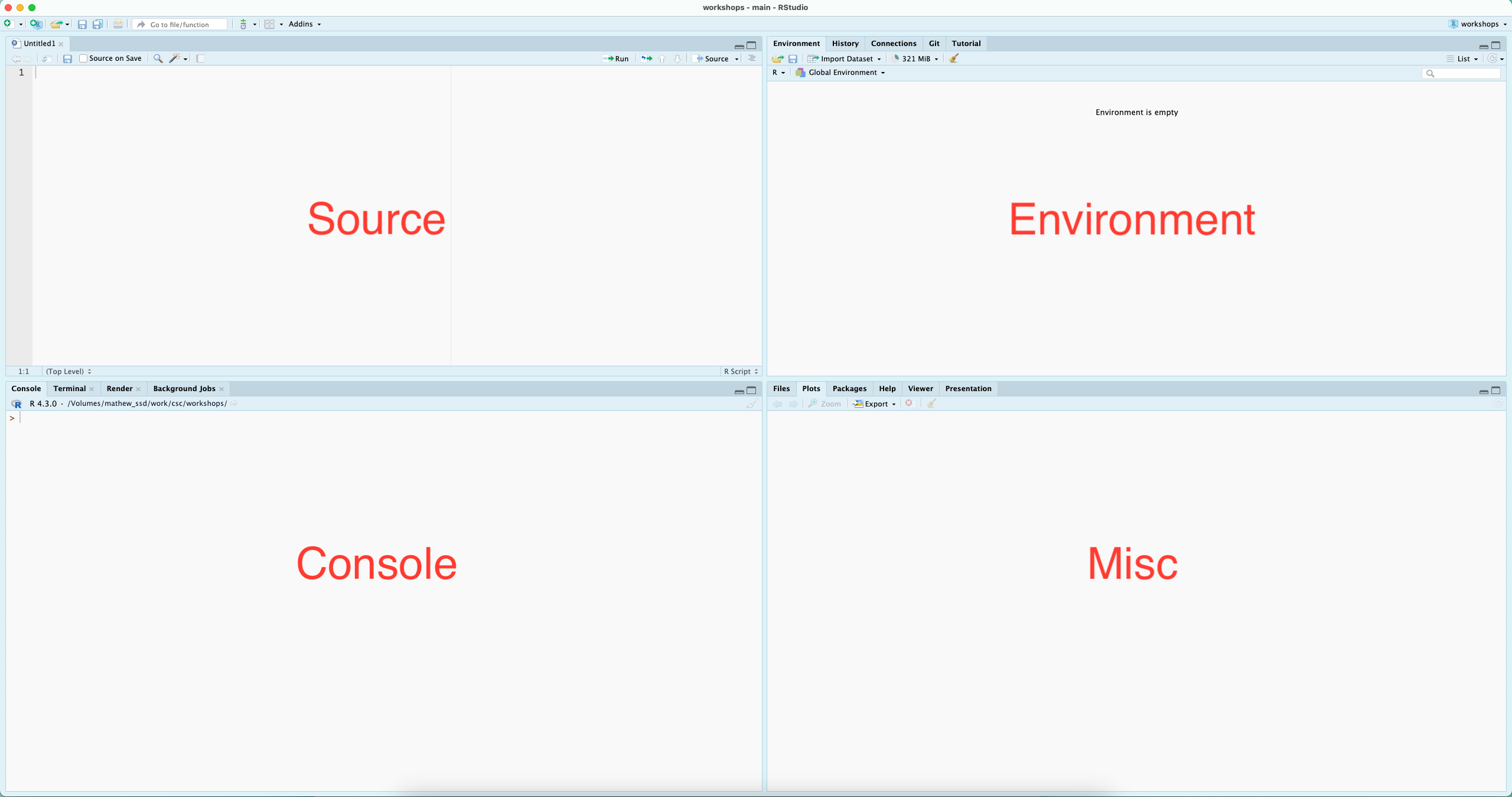
R is great for interactive computational analysis, allowing for easy exploration and iteration. Using an IDE - Integrated Development Environment - such as RStudio, facilitates this interactivity, providing you with easy access to a place to quickly code (the console), a place to write saveable scripts (source editor), a place to view the objects that you create (environment pane), and a place to interact with your file system, visual outputs from your code, and help documentation (the miscellaneous pane, for lack of a better word).
Simple Math
At it’s most basic, R is a glorified calculator, capable of any operation might wish to throw at it…
# addition
2 + 2
## [1] 4
# subtraction
3 - 2
## [1] 1
# mulitplication
3 * 3
## [1] 9
# division
4 / 2
## [1] 2
# square root
sqrt(9)
## [1] 3
# log 10
log10(100)
## [1] 2
Functions
At least initially, everything you do in R will be applying functions to data. In the above section, the mathematical operators, sqrt(), and log10(), are all functions. Functions take in data (or values) and process them, providing an output. The output is displayed in your console by default.
# c() is a common function for concatenating things together
c(1:10)
## [1] 1 2 3 4 5 6 7 8 9 10
Variables
While having outputs directed to the console is convenient for interactive analysis, often we need to store data and / or outputs for later use. We do this with variable assignmet, where the greater than and dash are used to assign the values (object) on the right to the name (variable) on the left.
my_variable <- c(1:10)
You can then recall the values (object) associated with your variable…
my_variable
## [1] 1 2 3 4 5 6 7 8 9 10
And plug it into functions, ie, do computations on it…
my_variable * 2
## [1] 2 4 6 8 10 12 14 16 18 20
When naming variables in R, keep in mind that variable names:
- Should first and foremost be meaningful. This is not a rule, just best practice.
- Cannot start with a number or a dot followed by a number.
- Cannot contain spaces or hyphens.
- Can contain letters, numbers, dots, and underscores.
Additionally, some words are reserved and cannot be used, such as if and for. More details can be found with
?make.names
Data Types & Structures
Data Types
Data types are elemental data constructs that R is able to distinguish between. The most common data types in R are numeric, character, and boolean. These come with intrinsic properties, for example, numeric data can be computed (added, divided, etc), character data can be strung together (character data, especially groups of characters are referred to as strings), and boolean data facilitates working with dichotomous values.
booleandata are generally referred to aslogical.numericdata are subdivided intodoubleandinteger; the difference is generally of little significance, as R manages the distinctions for you, but be wary if you’re dealing with particularly large numbers.characterdata always needs to be wrapped in single or double quotations.
The function typeof(), will tell you what data type you have…
typeof(2)
## [1] "double"
typeof("a")
## [1] "character"
typeof(TRUE)
## [1] "logical"
Data Structures
Data structures are ways to hold multiple pieces of data together in a meaningful way. R has four convenient ways of storing multiple pieces of data: vectors, matrices, data frames, and lists.
Vectors
The most basic is a vector. In fact, everything in R is a vector, and all other data structures are composed of vectors in various ways. It’s convenient to think of a vector as a simple list of like things; everything in a vector needs to be of the same data type. So, a vector can be:
- numeric, holding numeric data;
- character, holding character data; or
- logical, holding boolean data.
A vector can be created with c()
# numeric vector
c(1:10)
## [1] 1 2 3 4 5 6 7 8 9 10
# character vector
c("a", "b", "c")
## [1] "a" "b" "c"
# logical vector
c(TRUE, TRUE, FALSE)
## [1] TRUE TRUE FALSE
Matrices
A matrix is a vector with 2 dimensions; while a vector only has a length, a matrix is a grid with both length and width, or alternatively, rows and columns.
You can create a matrix with the matrix() function, providing it first with a series of values followed by an argument for the number of rows or columns you’d like.
matrix(1:10, nrow = 2)
##      [,1] [,2] [,3] [,4] [,5]
## [1,]    1    3    5    7    9
## [2,]    2    4    6    8   10
matrix(1:10, ncol = 2)
##      [,1] [,2]
## [1,]    1    6
## [2,]    2    7
## [3,]    3    8
## [4,]    4    9
## [5,]    5   10
A matrix must be perfectly rectangular, that is, each column must be of equal length. R will recycle values to ensure this condition is met.
# R will recycle the 1 to complete the rectangle
matrix(1:11, ncol = 2)
## Warning in matrix(1:11, ncol = 2): data length [11] is not a sub-multiple or
## multiple of the number of rows [6]
##      [,1] [,2]
## [1,]    1    7
## [2,]    2    8
## [3,]    3    9
## [4,]    4   10
## [5,]    5   11
## [6,]    6    1
A matrix must also be atomic - the data type must be the same throughout.
Data frames
In general, these will be the most likely data structures that you’ll encounter and the most familiar, as they are designed for tabular data and look like a spreadsheet.
Data frames are collections of vectors, where each vector must be of the same length, but can be of a different data type. If you import data from an Excel or csv file, these will be read in as a data frame. You can also create them with the data.frame() function.
data.frame(var_1 = letters,
           var_2 = 1:26)
##    var_1 var_2
## 1      a     1
## 2      b     2
## 3      c     3
## 4      d     4
## 5      e     5
## 6      f     6
## 7      g     7
## 8      h     8
## 9      i     9
## 10     j    10
## 11     k    11
## 12     l    12
## 13     m    13
## 14     n    14
## 15     o    15
## 16     p    16
## 17     q    17
## 18     r    18
## 19     s    19
## 20     t    20
## 21     u    21
## 22     v    22
## 23     w    23
## 24     x    24
## 25     y    25
## 26     z    26
Lists
Like data frames, lists are collections of vectors. However, unlike data frames, the length of these vectors can change. So far, this is the only non-rectangular data structure that we have to work with.
If you are importing tabular data, you are unlikely to create a list yourself, however, when performing operations (using functions) on your data, the output, or result, might be in the form of a list. For demonstration puropses, a list can be created with the list() function.
list(item_1 = letters,
     item_2 = 1:10,
     item_3 = c(TRUE, FALSE))
## $item_1
##  [1] "a" "b" "c" "d" "e" "f" "g" "h" "i" "j" "k" "l" "m" "n" "o" "p" "q" "r" "s"
## [20] "t" "u" "v" "w" "x" "y" "z"
##
## $item_2
##  [1]  1  2  3  4  5  6  7  8  9 10
##
## $item_3
## [1]  TRUE FALSE
Identifying Data Structures
The function class() will tell you what kind of structure your data are held in.
class(), when called on a vector, will report on the data type, which should be read as the type of atomic vector you have. An array is a multi-dimensional vector, a matrix is the special case where there are only two dimensions.
class(c(1:10))
## [1] "integer"
class(matrix(1:10, ncol = 2))
## [1] "matrix" "array"
class(data.frame(var_1 = letters,
           var_2 = 1:26))
## [1] "data.frame"
class(list(item_1 = letters,
     item_2 = 1:10,
     item_3 = c(TRUE, FALSE)))
## [1] "list"
Getting Help
There are five primary ways to get help (other than asking a friend) with R.
The first is with the built in documentation, which can be accessed by preceding a function name with a ?.
?sqrt()
These pages can be both enlightening and frustrating, as they assume some pre-existing familiarity with certain concepts as well as reading this kind of documentation.
The second is from forums. These are useful when you have a specific issue that you’re trying to resolve, and can often provide a quick fix, but the explanations also often require a degree of familiarity to make sense.
The third is blog posts and course supports posted on line. These generally provide more context than forum posts, and are useful when tyring to learn a new approach or a new library.
The fourth is journal publications that accompany the release of specific packages or libraries. These offer in depth descriptions of the packages and their arguments, often with examples.
The fourth is more in depth texts. Many of these are available publicly online, and include titles such as:
- aRrgh: a newcomer’s (angry) guide to R, by Tim Smith and Kevin Ushey - http://arrgh.tim-smith.us/
- YaRrr! The Pirate’s Guide to R, by Nathaniel D. Phillips - https://bookdown.org/ndphillips/YaRrr/
- R for Graduate Students, by Wendy Huynh. - https://bookdown.org/yih_huynh/Guide-to-R-Book/
- Advanced R, by Hadley Wickham - http://adv-r.had.co.nz/Introduction.html
And through the library, the O’Reilly platform hosts a plethora of titles related to R.
Test your R Might!
Here are some examples for you to look at and challenge yourself, ensuring you now have a better understanding of today’s session and how R works!
-
Create the vector [1, 2, 3, 4, 5, 6, 7, 8, 9, 10] in three ways: once using
c(), once usinga:b, and once usingseq(). -
Create the vector [0, 5, 10, 15] in 3 ways: using
c(),seq()with abyargument, andseq()with alength.outargument. -
Create a data frame named
dfwith the following columns:ID(1 to 10),Name(a character vector of names), andScore(randomly generated values between 50 and 100). Then, add a new columnPassthat indicates whether the score is above 60.