workshops

Last Updates: 2023-10-19

Missing Values

is.na()

Missing values in R are coded as NA, a special value in R. When importing or tyding your data, it’s important to ensure that you’re properly identifying missing values, and handling them with the arguments na.strings, if using read.csv(), or na, if using read_csv().

na_values <- c("NA", "NULL", "", " ")
data_gapminder <- read.csv("../data/gapminder_nas.csv", na.strings = na_values)

With the data loaded, we can investigate missing values. is.na() returns a logical vector, TRUE for NA, otherwise FALSE. This is easiest with a single vector…

# get colnames
colnames(data_gapminder)

## [1] "country"   "continent" "year"      "lifeExp"   "pop"       "gdpPercap"

# generate logical vector
missing_pop <- is.na(data_gapminder$pop)
typeof(missing_pop)

## [1] "logical"

head(missing_pop)

## [1] FALSE FALSE FALSE FALSE FALSE FALSE

The logical vector on it’s own, is not super helpful. We can generate counts of the TRUE values by summing the number of TRUE instances in missing_pop…

sum(missing_pop)

## [1] 223

We can do this more interactively with

sum(is.na(data_gapminder$pop))

## [1] 223

Complete Cases

Another point of interest in looking at missing values is to explore the number of observations for which no data are missing, which can be done with complete.cases(). Similar to is.na(), complete.cases() returnds a logical vector…

complete_gapminder <- complete.cases(data_gapminder)
typeof(complete_gapminder)

## [1] "logical"

We can get a count, like before

sum(complete_gapminder)

## [1] 853

And for use later, when subsetting, we can also generate a vector of those which are complete, identified by their index number. This is done with which()

# first few index numbers of comlpete cases
head(which(complete_gapminder))

## [1]  2  3  4  5  8 12

Unique values & duplicates

unique(), returns a vector of unique values…

unique(data_gapminder$continent)

## [1] "Asia"     "Europe"   "Africa"   "Americas" "Oceania"

duplicated() returns a logical vector, TRUE for values (of a vector) or rows (of a data frame) that are duplicates, FALSE if they are unique. Since the first instance of a value is unique, the first value will return FALSE, and any subsequent duplicates will return TRUE.

# on a vector
head(duplicated(data_gapminder$continent))

## [1] FALSE  TRUE  TRUE  TRUE  TRUE  TRUE

# there are 5 unique continents and 1699 duplicates
sum(duplicated(data_gapminder$continent))

## [1] 1699

# on a data frame
head(duplicated(data_gapminder))

## [1] FALSE FALSE FALSE FALSE FALSE FALSE

# there are no duplicate values
sum(duplicated(data_gapminder))

## [1] 0

Descriptive Statistics

Basic stats fucntions in R generally do not remove NA values by default, and if your data has NA values, they will return NA. You can avoid these errors with na.rm = TRUE as an argument.

Number of Observations

The number of values in a single vector can be derived with length()

length(data_gapminder$country)

## [1] 1704

When used on a data frame, however, length() returns the number of columns…

length(data_gapminder)

## [1] 6

When working with data frames, it is preferable to use nrow() and ncol() for the number of rows and columns, respectively.

ncol(data_gapminder)

## [1] 6

nrow(data_gapminder)

## [1] 1704

Range

The range of your data can be calculated with range().

range(data_gapminder$year, na.rm = TRUE)

## [1] 1952 2007

If you’re only interested in the min or max values individually, this can be pulled with min() and max() respectively.

min(data_gapminder$year, na.rm = TRUE)

## [1] 1952

max(data_gapminder$year, na.rm = TRUE)

## [1] 2007

Mean & Median

The mean and median are calculated with mean() and median() respectively…

mean(data_gapminder$lifeExp, na.rm = TRUE)

## [1] 58.9021

median(data_gapminder$gdpPercap, na.rm = TRUE)

## [1] 3242.531

Variance and Standard Deviation

The variance and SD are calculated with var() and sd()…

var(data_gapminder$lifeExp, na.rm = TRUE)

## [1] 165.1613

sd(data_gapminder$lifeExp, na.rm = TRUE)

## [1] 12.85151

Quantiles

Quantiles can be derived with quantile(), which defaults to the max, min and interquartiles.

quantile(data_gapminder$gdpPercap, na.rm = TRUE)

##          0%         25%         50%         75%        100% 
##    241.1659   1147.3888   3242.5311   8533.0888 113523.1329

Summaries

Much of the above can be gathered all at once if needed with summary(). summary() can be run on a single vector, or on an entire data frame…

summary(data_gapminder$gdpPercap)

##     Min.  1st Qu.   Median     Mean  3rd Qu.     Max.     NA's 
##    241.2   1147.4   3242.5   6839.5   8533.1 113523.1      219

summary(data_gapminder)

##    country           continent              year         lifeExp     
##  Length:1704        Length:1704        Min.   :1952   Min.   :23.60  
##  Class :character   Class :character   1st Qu.:1962   1st Qu.:47.83  
##  Mode  :character   Mode  :character   Median :1977   Median :59.63  
##                                        Mean   :1979   Mean   :58.90  
##                                        3rd Qu.:1992   3rd Qu.:70.60  
##                                        Max.   :2007   Max.   :82.60  
##                                        NA's   :217    NA's   :192    
##       pop              gdpPercap       
##  Min.   :6.001e+04   Min.   :   241.2  
##  1st Qu.:2.736e+06   1st Qu.:  1147.4  
##  Median :6.703e+06   Median :  3242.5  
##  Mean   :2.835e+07   Mean   :  6839.5  
##  3rd Qu.:1.836e+07   3rd Qu.:  8533.1  
##  Max.   :1.319e+09   Max.   :113523.1  
##  NA's   :223         NA's   :219

A better summary would come from properly denoted data types…

# summary with the first three columns classed as categorical data
summary(data_gapminder)

##         country        continent        year        lifeExp     
##  Afghanistan:  12   Africa  :624   1962   :132   Min.   :23.60  
##  Albania    :  12   Americas:300   1957   :128   1st Qu.:47.83  
##  Algeria    :  12   Asia    :396   1967   :127   Median :59.63  
##  Angola     :  12   Europe  :360   1952   :125   Mean   :58.90  
##  Argentina  :  12   Oceania : 24   1982   :125   3rd Qu.:70.60  
##  Australia  :  12                  (Other):850   Max.   :82.60  
##  (Other)    :1632                  NA's   :217   NA's   :192    
##       pop              gdpPercap       
##  Min.   :6.001e+04   Min.   :   241.2  
##  1st Qu.:2.736e+06   1st Qu.:  1147.4  
##  Median :6.703e+06   Median :  3242.5  
##  Mean   :2.835e+07   Mean   :  6839.5  
##  3rd Qu.:1.836e+07   3rd Qu.:  8533.1  
##  Max.   :1.319e+09   Max.   :113523.1  
##  NA's   :223         NA's   :219

Visualizing Distributions

Plotting for presentation will be covered in greater detail in a future session.

Basic plotting for distribution analysis is relatively straight forward in base R.

Distribution of a Single Variable

Histograms

You can plot a basic histogram with hist()

hist(data_gapminder$gdpPercap)

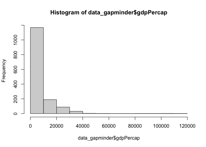
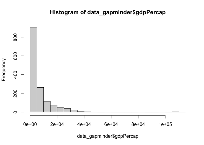
And you can increase the ‘buckets’ with the breaks argument

hist(data_gapminder$gdpPercap, breaks = 30)

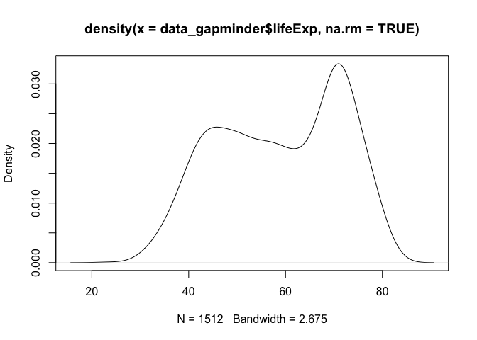
Density Plots

A density plot can be generated with plot(), but requires the extra step of computing the density of the data with the density() function first

dens <- density(data_gapminder$lifeExp, na.rm = TRUE)
plot(dens)

Distribution of Two Variables

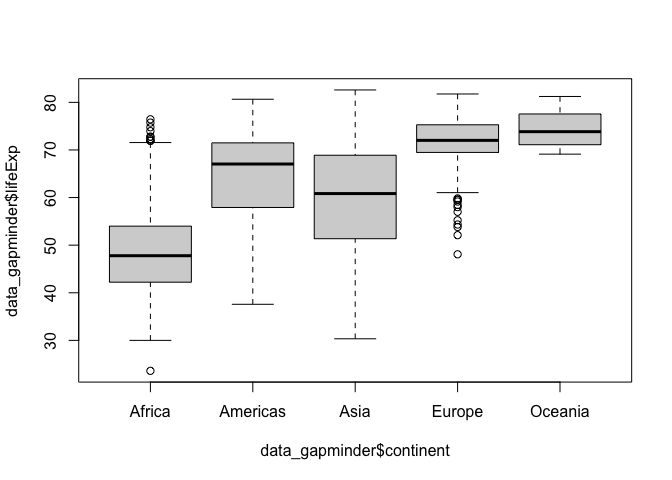
Box Plots

boxplot() allows you to facet one variable by another using a tilde ~ to define the relationship

boxplot(data_gapminder$lifeExp ~ data_gapminder$continent)

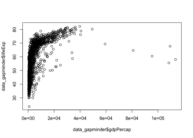
Scatter Plots

plot() by default assumes a single variable as in the earlier example, but will generate a scatter plot if provided with two variables, the first assigned to the x-axis, the second to the y-axis.

plot(x = data_gapminder$gdpPercap, y = data_gapminder$lifeExp)

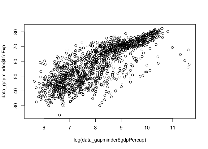
You can also transform you data within the function for quick investigation

# log transform gdp per capita
plot(x = log(data_gapminder$gdpPercap), y = data_gapminder$lifeExp)