workshops
Exploratory Data Anaysis
Let’s import our library and data set.
#import all libraries required for this data.
import pandas as pd
import numpy as np
import matplotlib.pyplot as plt
import seaborn as sns
# Reading CSV files from GitHub
gapminder = pd.read_csv('https://raw.githubusercontent.com/csc-ubc-okanagan/workshops/a091bc6eae8b9045866c28dbd1848c7e072db5b1/data/gapminder.csv')
gapminder_nas = pd.read_csv('https://raw.githubusercontent.com/csc-ubc-okanagan/workshops/a091bc6eae8b9045866c28dbd1848c7e072db5b1/data/gapminder_nas.csv')

# Reading Excel file from GitHub
gapminder_xlsx = pd.read_excel('https://raw.githubusercontent.com/csc-ubc-okanagan/workshops/a091bc6eae8b9045866c28dbd1848c7e072db5b1/data/gapminder.xlsx', engine='openpyxl')
# Exporting CSV files
gapminder.to_csv('gapminder.csv', index=False)
gapminder_nas.to_csv('gapminder_nas.csv', index=False)

# Exporting Excel file
gapminder_xlsx.to_excel('gapminder.xlsx', index=False, engine='openpyxl')
Handling Missing Values with Pandas
Datasets often have missing or placeholder values. Pandas, a Python data manipulation library, offers tools to address this. Using the na_values parameter when reading a dataset, like “gapminder_nas.csv”, enables Pandas to recognize placeholders such as “NA”, “NULL”, or empty spaces, and treat them as NaN. This simplifies subsequent data cleaning and analysis.
# Assuming you've read in the data
na_values = ["NA", "NULL", "", " "]
data_gapminder = pd.read_csv("gapminder_nas.csv", na_values=na_values)
data_gapminder.head()
| country | continent | year | lifeExp | pop | gdpPercap | |
|---|---|---|---|---|---|---|
| 0 | Afghanistan | Asia | 1952.0 | NaN | 8425333.0 | 779.445314 |
| 1 | Afghanistan | Asia | 1957.0 | 30.332 | 9240934.0 | 820.853030 |
| 2 | Afghanistan | Asia | 1962.0 | 31.997 | 10267083.0 | 853.100710 |
| 3 | Afghanistan | Asia | 1967.0 | 34.020 | 11537966.0 | 836.197138 |
| 4 | Afghanistan | Asia | 1972.0 | 36.088 | 13079460.0 | 739.981106 |
Checking for Missing Values
Now we will determine if there are any missing values in the ‘pop’ column of the data_gapminder dataframe. The isna() function is used to create a boolean series, missing_pop, where True denotes a missing value and False signifies a present value. By displaying the first few entries with head() and summing up the True values, we can gain a quick insight into both the presence and the total count of missing values in that column.
data_gapminder.info()
<class 'pandas.core.frame.DataFrame'>
RangeIndex: 1704 entries, 0 to 1703
Data columns (total 6 columns):
 #   Column     Non-Null Count  Dtype
---  ------     --------------  -----
 0   country    1704 non-null   object
 1   continent  1704 non-null   object
 2   year       1487 non-null   float64
 3   lifeExp    1512 non-null   float64
 4   pop        1481 non-null   float64
 5   gdpPercap  1485 non-null   float64
dtypes: float64(4), object(2)
memory usage: 80.0+ KB
# Missing Values
missing_pop = data_gapminder['pop'].isna()
print(missing_pop.head())
print(sum(missing_pop))
0    False
1    False
2    False
3    False
4    False
Name: pop, dtype: bool
223
Filter missing values
Now let’s filter the data_gapminder dataframe to retain only the rows that have no missing values across all columns. This is accomplished using the dropna() method, which removes any row containing a NaN value. The result will be stored in the complete_gapminder dataframe. By printing the length of this filtered dataframe, we can determine the number of complete cases, i.e., rows without any missing values, in our dataset.
# Complete Cases
complete_gapminder = data_gapminder.dropna()
print(len(complete_gapminder))
853
Quick Descriptive Statistics
- The total number of entries in the ‘country’ column.
# Descriptive Statistics
# Number of Observations
print(len(data_gapminder['country']))
1704
Dimentions of dataset
- The overall dimensions of the dataframe, indicating the number of rows and columns.
print(data_gapminder.shape) # (number of rows, number of columns)
(1704, 6)
Minimum and Maximum
- Display the minimum and maximum values of the ‘year’ column in the data_gapminder dataframe, effectively showing the range of years covered by the dataset.
#describe the following # Range
print(data_gapminder['year'].min())
print(data_gapminder['year'].max())
1952.0
2007.0
Mean and Median
- Calculate and print the average (mean) value for the ‘lifeExp’ (life expectancy) column and the median (middle) value for the ‘gdpPercap’ (GDP per capita) column in the data_gapminder dataframe.
# Mean & Median
print(data_gapminder['lifeExp'].mean())
print(data_gapminder['gdpPercap'].median())
58.902098095238095
3242.531147
Variance and Standard Deviation
- Calcualte and display the variance and standard deviation for the ‘lifeExp’ (life expectancy) column in the data_gapminder dataframe. Variance measures how spread out the numbers in a dataset are, while the standard deviation indicates the average amount the values deviate from the mean.
# Variance and Standard Deviation
print(data_gapminder['lifeExp'].var())
print(data_gapminder['lifeExp'].std())
165.1612971475914
12.851509527973413
Quantiles
- Calcualte and display the quantiles for the ‘gdpPercap’ (GDP per capita) column in the data_gapminder dataframe. Specifically, calculate the minimum (0% quantile), first quartile (25% quantile), median (50% quantile), third quartile (75% quantile), and maximum (100% quantile) values, providing insights into the data’s distribution and spread.
# Quantiles
print(data_gapminder['gdpPercap'].quantile([0, 0.25, 0.5, 0.75, 1]))
0.00       241.165876
0.25      1147.388831
0.50      3242.531147
0.75      8533.088805
1.00    113523.132900
Name: gdpPercap, dtype: float64
Statistical Summary
Now let’s create statistical summary for the ‘gdpPercap’ column and the entire data_gapminder dataframe.
For the ‘gdpPercap’ column, it presents metrics like count, mean, standard deviation, minimum, 25th percentile, median, 75th percentile, and maximum. For the entire dataframe, it provides a similar statistical breakdown for all numerical columns, giving a comprehensive view of the dataset’s characteristics.
# Summaries
print(data_gapminder['gdpPercap'].describe())
print(data_gapminder.describe())
count      1485.000000
mean       6839.475803
std        9686.630785
min         241.165876
25%        1147.388831
50%        3242.531147
75%        8533.088805
max      113523.132900
Name: gdpPercap, dtype: float64
              year      lifeExp           pop      gdpPercap
count  1487.000000  1512.000000  1.481000e+03    1485.000000
mean   1979.162071    58.902098  2.835264e+07    6839.475803
std      17.265521    12.851510  1.033339e+08    9686.630785
min    1952.000000    23.599000  6.001100e+04     241.165876
25%    1962.000000    47.831750  2.736300e+06    1147.388831
50%    1977.000000    59.625500  6.702668e+06    3242.531147
75%    1992.000000    70.596500  1.835666e+07    8533.088805
max    2007.000000    82.603000  1.318683e+09  113523.132900
Visualizing Data Distributions: Histogram
- Visualizes the distribution of the ‘gdpPercap’ column from the data_gapminder dataframe using a histogram. A histogram is a graphical representation that groups a dataset into bins and displays the frequency of data points within each bin. By executing this code, we will see a plot that offers insights into the spread and central tendencies of the GDP per capita values in the dataset.
# Visualizing Distributions
# Histograms
data_gapminder['gdpPercap'].hist()
plt.show()
Now let’s display a histogram of the ‘gdpPercap’ column from the data_gapminder dataframe with 30 bins, visualizing the distribution of GDP per capita values across these bins.
data_gapminder['gdpPercap'].hist(bins=30)
plt.show()
Density Plot
We can also generate a smooth density plot, visualizing the distribution of the ‘lifeExp’ column from the data_gapminder dataframe.
# Density Plots
data_gapminder['lifeExp'].plot(kind='density')
plt.show()

Boxplot
In the following code we will display a box plot comparing the distribution of ‘lifeExp’ values grouped by different ‘continent’ categories in the data_gapminder dataframe.
# Box Plots
data_gapminder.boxplot(column='lifeExp', by='continent')
plt.show()
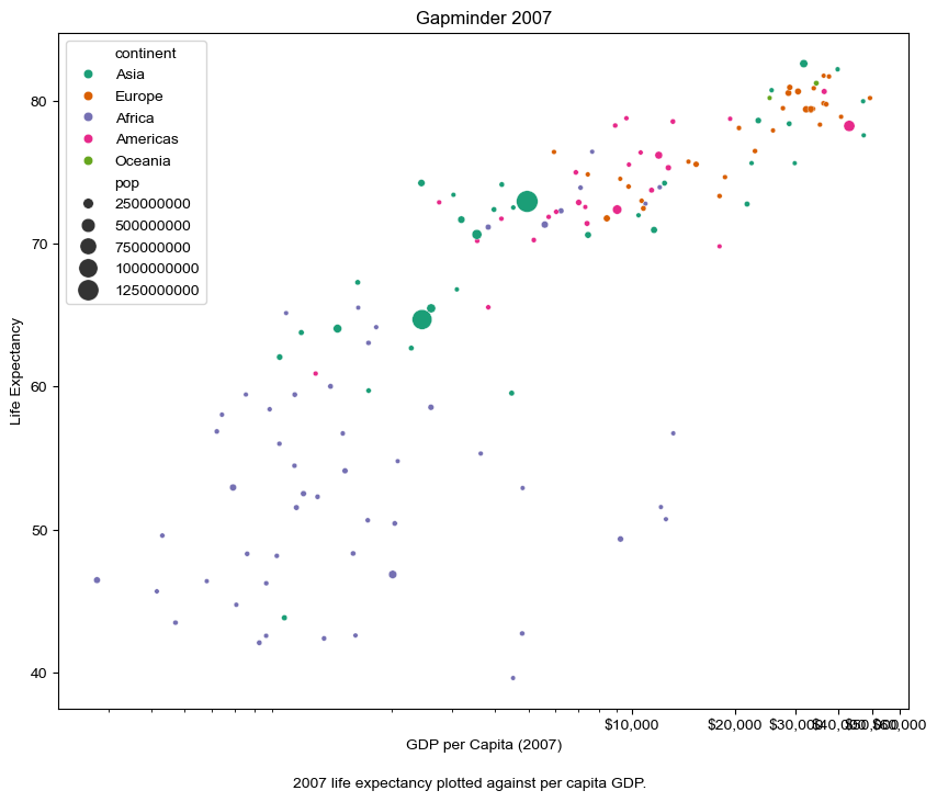
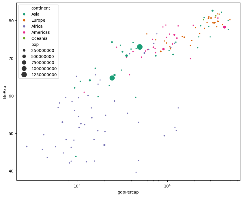
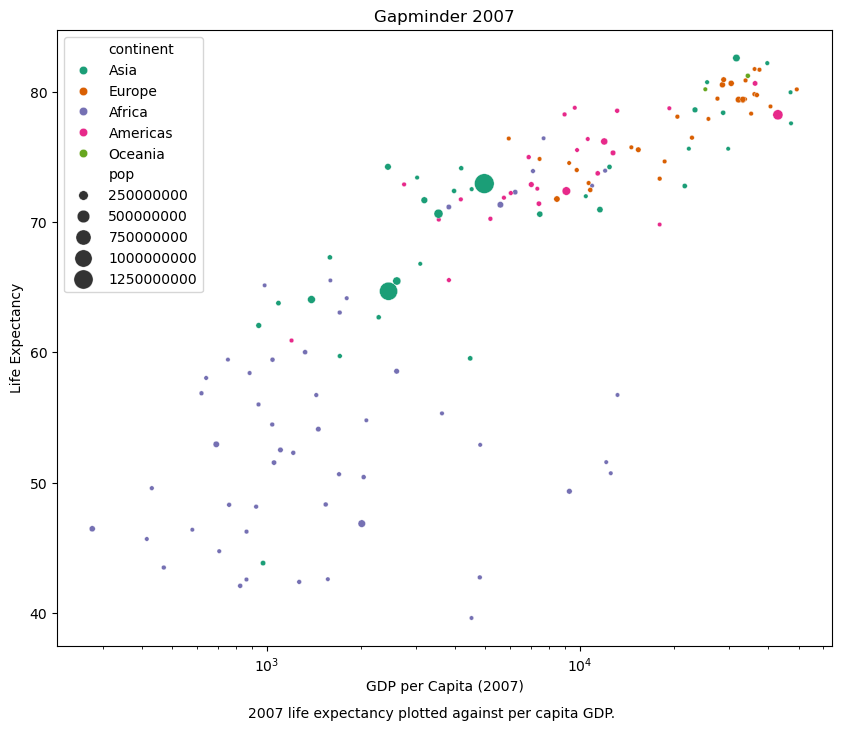
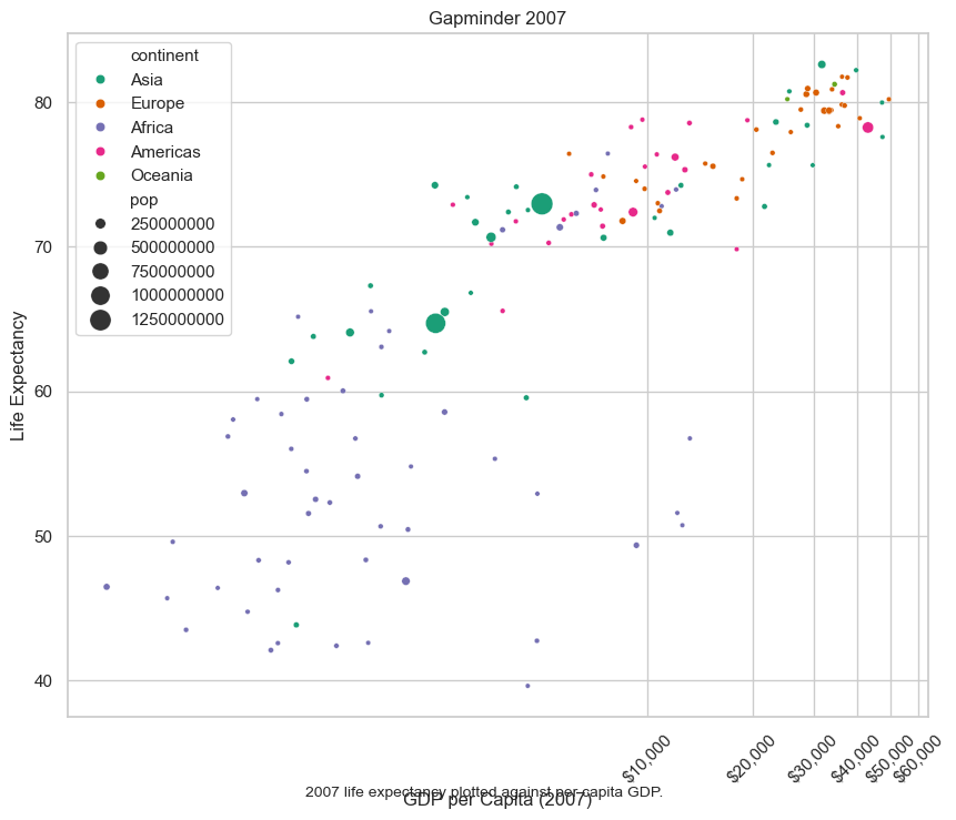
Scatter plots
Finally, we will generate two scatter plots:
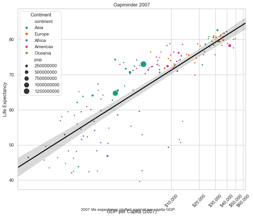
- The first scatter plot visualizes the relationship between ‘gdpPercap’ and ‘lifeExp’ in the data_gapminder dataframe.
- The second scatter plot does the same but with the ‘gdpPercap’ values log-transformed, allowing for clearer visualization of data spanning several orders of magnitude.
# Scatter Plots
data_gapminder.plot(x='gdpPercap', y='lifeExp', kind='scatter')
plt.show()
- Caculate the natural logarithm of the gdpPercap column in the data_gapminder DataFrame and stores the result in a new column named log_gdpPercap. Then, plot a scatterplot comparing this log-transformed GDP per capita against life expectancy (lifeExp).
plt.scatter(x=np.log(data_gapminder['gdpPercap']), y=data_gapminder['lifeExp'])
plt.show()
References
Gapminder Dataset
Python
NumPy
Pandas
Seaborn
Matplotlib