Overview of spectral analysis

What do ghosts, fourier analysis and landscape structure all have in common? Honestly…not much, but I’m here to talk to you about most of those topics anyway! Enter spectral analysis 👻.

Spectral analysis is the process of taking complex and signals (e.g., sound waves, images, or even landscape composition via rasters) and decomposing them into into periodic functions (i.e., sine and cosine waves) that can be more easily analyzed. Although there are many uses for spectral analysis, in this blog post I will just examine one particular use in the context of ecology–analyzing landscape structure. I probably don’t need to tell you dear reader that habitat (and thereby landscape structure) is a critical to an animal’s ability to thrive and reproduce. As such, it’s fundamental for wildilfe managers to understand how landscape structure (and our decisions to manage or alter that structure) may or may not impact the wild populations we care about!

Motivation aside spectral analysis we need a landscape. I’ll quickly go ahead and generate one with a handy function that generates landscapes with Gaussian random fields (GRFs).

 1
 2
 3
 4
 5
 6
 7
 8
 9
10
11
12
13


generate_grf_landscape <- function(a, size, matrix = TRUE){
    grid <- expand.grid(x = 1:size, y = 1:size)
    sp::coordinates(grid) <- ~ x + y
    sp::gridded(grid) <- TRUE
    vgm_mod <- gstat::vgm(psill = 1, model = "Exp", range = a, nugget = 0)
    g <- gstat(formula = z ~ 1, locations = ~ x + y, dummy = TRUE, beta = 0, model = vgm_mod, nmax = 20)
    sim <- predict(g, grid, nsim = 1)
    if(matrix){
        return(matrix(sim$sim1, nrow = size, ncol = size))
    }else{
        return(rast(matrix(sim$sim1, nrow = size, ncol = size)))
    }
}

Let’s start off by generating a few landscapes with different range parameters (a).

1
2
3
4
5
6
7


grf_range_values <- c(1, 10, 30) # definitely play around with these
# stick our landscapes into a list for convenience
# this generates a landscape for each range parameter `a` of size 100
land_list <- purrr::map(
    setNames(grf_range_values, grf_range_values),
    ~ rast(generate_grf_landscape(a = .x, size = 100))
)

1
2
3


## [using unconditional Gaussian simulation]
## [using unconditional Gaussian simulation]
## [using unconditional Gaussian simulation]

 1
 2
 3
 4
 5
 6
 7
 8
 9
10
11


# helper function
rast_to_df <- function(name, list) {
  # Works for SpatRaster with 1 layer
  df <- as.data.frame(list[[name]], xy = TRUE, na.rm = FALSE)
  names(df) <- c("Easting", "Northing", "value")
  df$a <- name
  df
}
# now we want to take this and turn it into a list of dataframes for easy plotting
# using ggplot
rast_df_list <- lapply(names(land_list), rast_to_df, list = land_list)

Note that I assumed we were only working with square matrices here…this is almost never the case in real data, but it’s an easy fix and makes things look neater for demonstration. Let’s go ahead and generate (and visualize 🔎) what the parameter a does…

 1
 2
 3
 4
 5
 6
 7
 8
 9
10
11
12
13
14
15
16
17
18
19
20
21
22
23
24
25
26
27
28
29
30
31
32
33
34
35
36


# i'll use these two little calls to get the maximum and miniumum values 
# over each one of our landscapes so that we can plot these on the same scale
g_max <- max(unlist(lapply(land_list, function(x) values(max(x))))) 
g_min <- max(unlist(lapply(land_list, function(x) values(min(x))))) 

# yet another custom function...sorry about all this
make_land_grid_plot <- function(dat, facet = NULL, g_min, g_max){
  if (!is.null(facet)) {
    dat <- dat %>% mutate(.facet_lab = paste0(facet, "==", .data[[facet]]))
  }
  p <- ggplot(dat, aes(Easting, Northing, fill = value)) +
    geom_raster() +
    coord_equal(expand = FALSE) +
    scale_fill_gradient(
      low = "black", high = "white",
      limits = c(g_min, g_max),
      name = NULL
    ) +
    labs(x = "Easting", y = "Northing") +
    scale_fill_gradientn(colours = terrain.colors(256)) +
    theme(
      panel.grid = element_blank(),
      strip.text = element_text(face = "bold"),
      axis.title = element_text(size = 12),
      legend.position = "right"
    )
  if (!is.null(facet)) {
    p <- p + facet_wrap(~ .facet_lab, labeller = label_parsed)
  }
  p
}
# let's do one more transform of our land dataframes so we can plug them into this
# function
land_df <- bind_rows(rast_df_list)
# now we can call our custom function to make the plots
land_plot <- make_land_grid_plot(land_df, facet = 'a', g_min = g_min, g_max = g_max)

1
2


## Scale for fill is already present.
## Adding another scale for fill, which will replace the existing scale.

OK great. That was a lot of work just to look at some GRFs…but hey–that’s ok.

1

land_plot

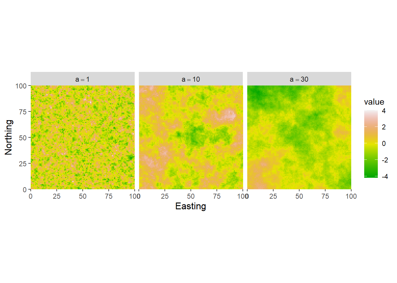OK so a couple of things to notice here. Remember the value `a` from the previous section? Just by inspection we can see that that the landscape is showing larger (more distinct) patches as the `a` parameter increases. In fancier terms landscape ecologists might say that the landscape is becoming more **autocorrelated**.

OK. OK. I hear what you’re thinking: “Alex, this blog post is about spectral analysis…and so far all we’ve done is plot some fancy looking fake lands…”, and you’d be correct! That is in fact all we’ve done, but now that we have some fake landscapes with varying degrees of structure (another way of talking about how autocorrelated your landscape is) we can start to analyze them…this time I promise.

To do spectral analysis let’s start with a concept…fourier transformations. I’m not scared…are you scared?…(ok I’m a little scared). So the big idea behind fourier transformation is that we can decompose a signal (again could be sound, habitat quality, or information compression in computer files) and decompose it into a set of basis functions. In essence what we’re doing is taking the original data and conducting what’s called a change of basis more on that here or you could check out Khan Academy. In short, a change of basis changes a dataset from one coordinate system to another one. In our case we take a system of coordinates from our landscape (could be real coordinates or the imaginary coordinates of the landscape I made up) and correlating each coordinate-pair to a value in the frequency domain. Let’s look at an example to make this more concrete.

Remember our handy landscapes from before?

1
2
3
4
5
6


# we'll just grab the grf land with "moderate" landscape autocorrelation
# a = 10
grf_a_10 <- land_list[[2]]
m <- terra::as.matrix(grf_a_10, wide = TRUE)
# let's run the fft to get the change of basis
freq_a_10 <- fft(m)

A couple of things to notice here. The object freq_a_10 is a an object of size 100, 100…the same dimensions as our grf landscape grf_a_10!! Coincidence…? Of course not. By the way you’re about to run into some math let’s refer to the landscape grf_a_10 as $ L $ from here on out, deal? Under the hood the function fft() (which stands for fast fourier transform by the way) from the R package stats is doing a change of basis from our original space (habitat values on a coordinate grid) to a totally different space (frequencies on a totally separate but equal grid of indices). The long and short of it is that for each cell in our landscape freq_a_10 finds the correlation between the landscape’s structure and a pair of cosine and sine functions.

Let’s zoom in a minute:

1

freq_a_10[1,3]

1

## [1] -671.5256-1029.249i

OK this is weird right? Why is there an i at the end of the number? And why are there two numbers here if it’s just correlation between two things? Well, the answer comes from the fourier transform itself. Let’s introduce $ \phi(r,c) $ (a basis function) which correlates our landscape index $ (r,c) $ (e.g., (1,0), (53, 15), …) to a value in the frequency space I mentioned earlier.

$$ \phi(r, c) = e^{2\cdot \pi \cdot i \cdot (\frac{kr}{N} + \frac{lc}{M})} (1) $$

So this gets me my correlating value in frequency space…but how do those values we saw in the object freq_a_10? Well I’m glad you asked…let’s calculate just one of those values as an example.

 1
 2
 3
 4
 5
 6
 7
 8
 9
10
11
12
13
14
15
16
17


# fft indexes starting at zero like most other things in computer science...
# except R. So we'll index the cell at [1,3] as [0,2]
k <- 0
l <- 2
N   <- 100
# generate a grid of cell indices
# notice that we're generating indicies on the frequency-domain scale
# i.e., 0-99
r_grid <- matrix(0:(N-1), nrow = N, ncol = N, byrow = FALSE)
c_grid <- matrix(0:(N-1), nrow = N, ncol = N, byrow = TRUE)
# phi_kl is just one of of these basis functions
phi_kl <- exp(2 * pi * 1i * (k * r_grid / N + l * c_grid / N))
# notice here that F_02 (which again corresponds to L[1,3] in our landscape-space)
# multiplies just one basis function phi_kl by the entire landscape 
# so we're getting a correlation between a single basis function and the entire
# domain we're interested in. Neat right?
F_02 <- sum(as.vector(m) * as.vector(phi_kl))

OK now if you and I haven’t completely lost our sanity…these values should be the same. Let’s check the value returned by fft -671.53 -1029.25i and the value we just calculated…-671.53 +1029.25i. Bingo! They’re the same!! So behind the scenes we’re just getting correlations between our landscape and the basis function. In math this means:

$$ F(k, l) = \sum_{r \in R} \sum_{c \in C} L(r,c) \cdot e^{2\cdot \pi \cdot i \cdot (\frac{k \cdot r}{N} + \frac{l \cdot c}{M})} \ (1) $$

And remember from Euler’s Formula we can write (1) as:

$$ \phi(r, c) = e^{2 \cdot \pi \cdot i \cdot (\frac{kr}{N} + \frac{lc}{M})} = \cos(2 \cdot \pi \cdot (\frac{kr}{N} + \frac{lc}{M})) + i \sin (2 \cdot \pi \cdot (\frac{kr}{N} + \frac{lc}{M})) $$

So, our landscape can be written as a decomposition of periodic basis vectors!! Yipee! This is cool…but what can we actually do with this? I’m glad you asked dear reader. One thing we can now do is numerically quantify the spatial structure of our landscape (or whatever else you personally happen to be interested in). Let’s learn about the utility of what we just did with one spectral measure of landscape structure the spectral centroid.

The Spectral Centroid

OK so now we have a frequency-domain representation of our landscape. Each cell F[k,l] in freq_a_10 tells us how strongly the landscape correlates with a wave that completes k cycles north-south and l cycles east-west. But we want a single number that summarises the dominant spatial scale—-this is where the spectral centroid comes in. Unfortunately, to do discuss the spectral centroid we’re going to have to introduce more actors into this play.

Remember how each of the components in our frequency matrix was an ugly complex number with two components (a real and imaginary one?). Yeah…let’s fix that. To do that I’ll introduce the power spectrum — the squared magnitude of each element of the frequency matrix from fft():

1
2
3


# power at each frequency — how strongly does the landscape correlate
# with each basis wave?
power <- Mod(freq_a_10)^2

The function Mod() collapses the complex number to a single amplitude. Squaring gives us power. Let take a gander at the cell we looked at earlier 1,510,299. See now it’s just a nice real number. We like real numbers.

Next we need to know the actual spatial frequency that each [k,l] index corresponds to — how many cycles per spatial unit, rather than per domain. To do that I will introduce the the dc component. The term dc actually stands for direct current borrowed from electrical engineering. In the out context it represents the zero-frequency term — the global mean habitat value across the landscape. It is directly analogous to (but not necessarily equal to) the nugget in a variogram or the intercept in regression analysis. But the dc component…it’s got to go.

 1
 2
 3
 4
 5
 6
 7
 8
 9
10


N <- nrow(m)
M <- ncol(m)

# frequency in cycles per cell, shifted so DC is at centre
freq_row <- (((seq_len(N) - 1) + floor(N/2)) %% N - floor(N/2)) / N
freq_col <- (((seq_len(M) - 1) + floor(M/2)) %% M - floor(M/2)) / M

# radial frequency magnitude at each [k,l] — combining both directions
freq_mat <- outer(freq_row, freq_col,
                  FUN = function(fr, fc) sqrt(fr^2 + fc^2))

Now the freq_mat component gets a little confusing. Since we’ve done a change of basis we are no longer working in euclidean space in the classical sense. We’re instead working in frequency or cycle space. So the euclidean distance we take sqrt(fr^2 + fc^2) is a measure of how many cycles distant each cell is from dc. This is our unit of measurement in this space. The radial frequency collapses the 2D frequency grid to a single number per cell — the combined spatial frequency regardless of direction. A wave with k=3, l=4 has the same radial frequency as k=4, l=3: they both complete the same number of cycles per unit, just oriented differently.

Now the spectral centroid (i.e., the power-weighted mean frequency):

$$ \omega = \frac{\sum_{k,l} f_{kl} \cdot P_{kl}}{\sum_{k,l} P_{kl}} $$

Here $ \omega $ is the term I’m using for the spectral centroid metric. Going from the numerator to the denominator. The $ \sum_{k,l}f_{kl} \cdot P_{kl} $ part. The sum is telling us that we want to continue the operation across all of the frequency-space indicies $ k,l $. At each of these indices we want to weight the frequency at a particular index $ f_{k,l} $ by it’s corresponding power $ P_{k,l} $. Remember that $ P_{k,l} $ is the square of the correlation matrix.

 1
 2
 3
 4
 5
 6
 7
 8
 9
10
11
12
13
14
15


# exclude DC component (zero frequency — just the landscape mean)
dc_mask <- freq_mat > 0
f_vals  <- freq_mat[dc_mask]
p_vals  <- power[dc_mask]

# power-weighted mean frequency — the "centre of mass" of the power spectrum.
# each frequency f_vals is weighted by how strongly the landscape correlates
# with that frequency (p_vals), so landscapes with coarse structure pull the
# centroid toward low frequencies and fine-grained landscapes pull it high.
f_centroid <- sum(f_vals * p_vals) / sum(p_vals)

# convert from frequency (cycles/cell) to wavelength (spatial units)
omega_sc <- 1 / f_centroid

cat("Spectral centroid wavelength:", round(omega_sc, 3), "spatial units\n")

1

## Spectral centroid wavelength: 13.541 spatial units

In short what we did:

fft()— correlate the landscape against every basis wave simultaneously
Mod()^2— how strong is each correlation? (power)
freq_mat— what frequency does each correlation correspond to? (ordered from zero outward)
sum(f*p)/p— or f_centroid where is the centre of mass of those correlations on the frequency axis (note we are talking about how many times the dominant pattern repeats per cell.).
1/f_centroid— convert to wavelength. f_centroid gives us a frequency, but remember that we’re interested in the scale of landscape autocorrelation, so we need to convert it to how many spatial units it takes to complete a cycle.

The final conversion from frequency to wavelength ($ \omega = 1/f $) gives us a spatial scale in the same units as the landscape. Let’s visualise what we just computed — the full radial power spectrum with the centroid marked:

 1
 2
 3
 4
 5
 6
 7
 8
 9
10
11
12
13
14
15
16
17
18


# bin power by radial frequency for a clean 1D plot
breaks  <- seq(0, max(f_vals), length.out = 60)
bin_idx <- cut(f_vals, breaks = breaks, include.lowest = TRUE)
binned  <- aggregate(p_vals ~ bin_idx, FUN = sum)
binned$freq_mid <- breaks[-length(breaks)] + diff(breaks) / 2

ggplot(binned, aes(freq_mid, p_vals)) +
  geom_col(fill = "grey70", width = diff(breaks)[1] * 0.9) +
  geom_vline(xintercept = f_centroid, 
             colour = "steelblue", linewidth = 1) +
  annotate("text", x = f_centroid, y = max(binned$p_vals) * 0.9,
           label = paste0("ω_sc = ", round(omega_sc, 2), " cells"),
           hjust = -0.1, colour = "steelblue", size = 3.5) +
  labs(x = "radial frequency (cycles / cell)",
       y = "summed power",
       title = "Radial power spectrum",
       subtitle = "Blue line = spectral centroid") +
  theme_bw()

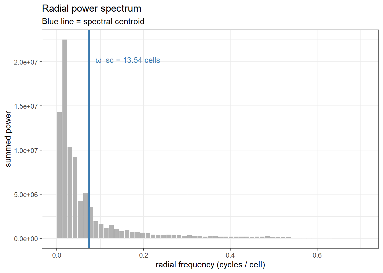OK great so for this particular GRF landscape this plot tells us that it takes it takes 14.09 units to complete a cycle on average. OK great, but let's jump back to the original problem.

Did we make a way to do spectral analysis

We wanted a property that would tell us the scale of landscape structure regardless of the actual structure itseslf…let’s see if we’ve actually done that. Let’s go ahead and write a convient function to summarise the steps we just took to calculate the spectral centroid.

 1
 2
 3
 4
 5
 6
 7
 8
 9
10
11
12
13
14
15
16
17
18
19
20
21
22
23
24
25
26
27
28
29
30
31
32
33
34
35
36
37
38
39
40
41
42
43
44
45


get_spectral_centroid <- function(rast) {
  # Get resolution (mean of x and y res to handle slight differences)
  res_x <- terra::xres(rast)
  res_y <- terra::yres(rast)
  cell_size <- mean(c(res_x, res_y))
  
  # extract matrix
  m <- terra::as.matrix(rast, wide = TRUE)
  
  nr <- nrow(m)
  nc <- ncol(m)
  
  # do our fast fourier transform from before
  ft    <- fft(m)
  # get the actual power or magnitude of the correlation between each basis
  # and the total landscape structure
  power <- Mod(ft)^2
  
  # Frequency arrays (cycles per cell), then convert to cycles per spatial unit
  freq_row <- (((seq_len(nr) - 1) + floor(nr / 2)) %% nr - floor(nr / 2)) / nr
  freq_col <- (((seq_len(nc) - 1) + floor(nc / 2)) %% nc - floor(nc / 2)) / nc
  
  # convert to cycles per spatial unit
  freq_row_spatial <- freq_row / res_y
  freq_col_spatial <- freq_col / res_x
  
  # build frequency magnitude grid (2D radial frequency in cycles / spatial unit)
  # remember these are our 'indicies' for our new domain
  freq_mat <- outer(freq_row_spatial, freq_col_spatial,
                    FUN = function(fr, fc) sqrt(fr^2 + fc^2))
  
  # exclude DC component 
  dc_mask <- freq_mat > 0
  f_vals  <- freq_mat[dc_mask]
  p_vals  <- power[dc_mask]
  
  f_centroid  <- sum(f_vals * p_vals) / sum(p_vals)
  1 / f_centroid
}
# before we do that let's generate a few more lands
grf_range_values <- c(1,3,4, 5, 6,7, 9, 10, 12, 13, 14, 15, 16, 17, 18, 19, 20, 21, 22, 23, 25, 27, 30)
land_list_ext <- land_list <- purrr::map(
    setNames(grf_range_values, grf_range_values),
    ~ rast(generate_grf_landscape(a = .x, size = 100))
)

 1
 2
 3
 4
 5
 6
 7
 8
 9
10
11
12
13
14
15
16
17
18
19
20
21
22
23


## [using unconditional Gaussian simulation]
## [using unconditional Gaussian simulation]
## [using unconditional Gaussian simulation]
## [using unconditional Gaussian simulation]
## [using unconditional Gaussian simulation]
## [using unconditional Gaussian simulation]
## [using unconditional Gaussian simulation]
## [using unconditional Gaussian simulation]
## [using unconditional Gaussian simulation]
## [using unconditional Gaussian simulation]
## [using unconditional Gaussian simulation]
## [using unconditional Gaussian simulation]
## [using unconditional Gaussian simulation]
## [using unconditional Gaussian simulation]
## [using unconditional Gaussian simulation]
## [using unconditional Gaussian simulation]
## [using unconditional Gaussian simulation]
## [using unconditional Gaussian simulation]
## [using unconditional Gaussian simulation]
## [using unconditional Gaussian simulation]
## [using unconditional Gaussian simulation]
## [using unconditional Gaussian simulation]
## [using unconditional Gaussian simulation]

1
2
3
4
5
6
7
8
9


# wrapper function so we can return the names of the list (a values)
# as elements of our dataframe
# it's a less fancy (and worse) version of the map approach i took above
process_lands <- function(x){
  data.frame(omega = get_spectral_centroid(land_list[[x]]),
    a_val = as.numeric(x)
  )
}
omega_dat <- bind_rows(lapply(names(land_list_ext), process_lands))

Here comes the kind of underwhelming finale.

1
2
3
4
5
6
7
8


ggplot(omega_dat, aes(x = a_val, y = omega)) +
  geom_point(size = 2.5) +
  geom_abline(slope = 1, intercept = 0, 
              linetype = "dashed", colour = "grey50") +
  labs(x = "true a (GRF range parameter)",
       y = expression(omega ~ "(cells per cycle)"),
       title = "Spectral centroid vs landscape scale") +
  theme_bw()

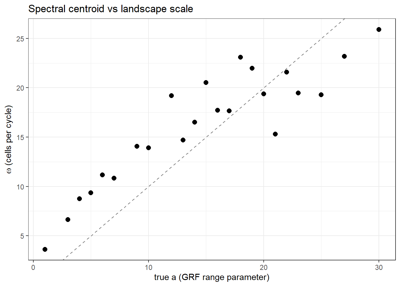Great! So it's admittedly not a perfect metric (there's some scatter about the one-one line), but considering the messiness of the dastaset we are getting a pretty good idea of the scale of the landscape in a way that's indepedent of the structure and values present!

References & Sources

Pebesma, E. & Bivand, R. (2023). Spatial Data Science: With Applications in R. Chapman and Hall. Boca Raton FL, United States. https://doi.org/10.1201/9780429459016. 10.1201/9780429459016. Taboga, Marco (2021). “Discrete Fourier Transform - Frequencies”, Lectures on matrix algebra. https://www.statlect.com/matrix-algebra/discrete-Fourier-transform-frequencies. Taboga, Marco (2021). “Discrete Fourier transform”, Lectures on matrix algebra. https://www.statlect.com/matrix-algebra/discrete-Fourier-transform. Taboga, Marco (2021). “Change of basis”, Lectures on matrix algebra. https://www.statlect.com/matrix-algebra/change-of-basis.