Meta-Analysis on Randomized Clinical Trials

Amir Golzan

In this part, we begin performing meta-analysis using the R language. If you are not familiar with R, you may refer to R for Data Science for a comprehensive introduction.

We will cover how to prepare data for import into RStudio, import the data, label it appropriately, and analyze it using meta-analysis codes.

Data Preparation

To perform meta-analysis, we first need to calculate the mean change and the Standard Deviation (SD) of the mean change for studies reporting only pre- and post-measurements. Additionally, we should label our data based on defined criteria (discussed further below) to prepare for subgroup analysis, which is critical in meta-analyses.

Let’s say we have extracted the following data from a study evaluating C-reactive protein (CRP) levels in blood after consuming Vitamin E (Ahmadi et al. 2013):

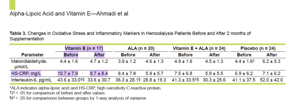
Our extracted data should look like this:

Mean_Pre_CRP	SD_Pre_CRP	Mean_Post_CRP	SD_Post_CRP	Mean_Change_CRP	SD_Change_CRP
10.7	7.9	8.7	8.4	?	?

Now we can calculate the mean change and SD of change using the following formulas:

Mean Change = \( Mean_{Post} - Mean_{Pre} \)
SD of Change = \( \sqrt{(SD_{Pre}^2 + SD_{Post}^2) - (2 \times r \times SD_{Pre} \times SD_{Post})} \)

The formula for calculating SD of Change requires a pre-post correlation (r). In general in RCTs, the Pre and Post Mean and SD, or Mean/SD changes are reported. However, if the latter are not, we need some way of estimating r. One way of doing this is to draw from an included study in which the authors do report r or SD of Change. If the SD of Change is reported, we can re-order the above formula to solve for r:

r: \( \frac{SD_{Pre}^2 + SD_{Post}^2 - SD_{change}^2}{2 \times SD_{Pre} \times SD_{Post}} \)

In our example the SD of change is not reported. Therefore, to calculate r, we use the following known study information (Pirhadi-Tavandashti et al. 2020):

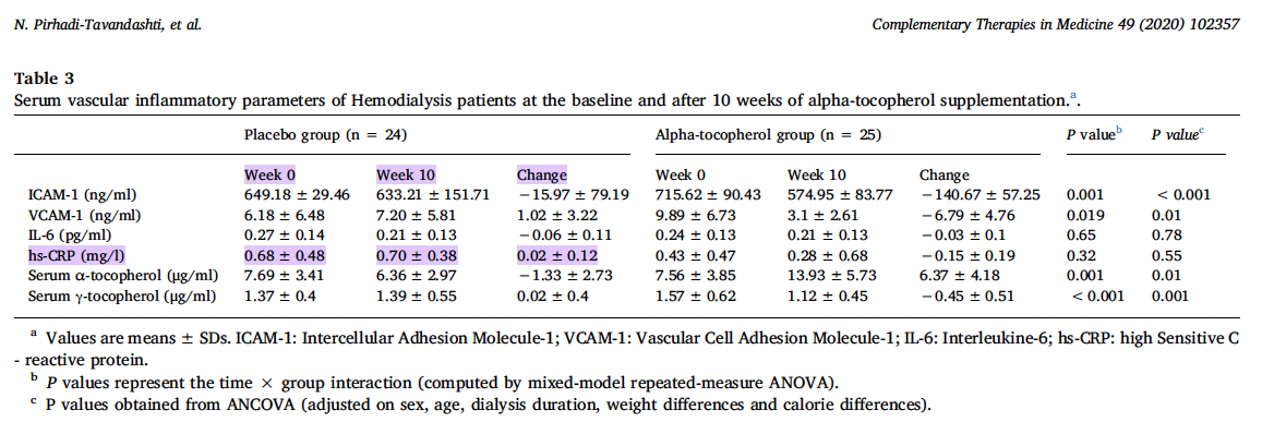
r: \( \frac{(0.48^2) + (0.38^2) - (0.12^2)}{2 \times 0.48 \times 0.38} = 0.98 \)

So in our example, we can assume r as 0.98.

SD change = \( \sqrt{((7.9^2) + (8.4^2)) - (2 \times 0.98 \times 7.9 \times 8.4)} = 1.70 \)

Considering these, we can now complete our table:

Mean_Pre_CRP	SD_Pre_CRP	Mean_Post_CRP	SD_Post_CRP	Mean_Change_CRP	SD_Change_CRP
10.7	7.9	8.7	8.4	-2	1.70

Note: You can study more about pre-post correlation here.

Subgroup Analysis Preparation

To perform subgroup analysis, we must assign codes to variables based on which we want to conduct the analysis. Commonly used variables include:

Gender
Dosage
Duration of intervention
Health status of individuals
Adjustment for baseline values
Study design
Adherence to the intervention

These variables can be coded as numeric values using mutate() function from dplyr package. For example, gender can be coded as: Both genders = Code 1, Male = Code 2, Female = Code 3.

For this part, we will use a sample data for demonstration. In this sample dataset, we want to understand how using Vitamin E affects the levels of CRP in blood. You can download the data to your local computer from Sample Data. The gender column indicates the gender of individuals researchers recruited in their study.

Let’s see how we can add a new column to our data, coding gender:

1
2
3
4
5
6
7
8


library(readr)
library(dplyr)

# Sample data
sample_data <- read_csv("sample_data.csv", show_col_types = FALSE) 

# Checking data
head(sample_data[, c("author name", "gender")])

1
2
3
4
5
6
7
8
9


## # A tibble: 6 × 2
##   `author name`       gender
##   <chr>               <chr> 
## 1 Dalgard et al. 2009 male  
## 2 Rafraf et al. 2012  female
## 3 Daud et al. 2013    both  
## 4 El-sisi et al. 2013 male  
## 5 Mah et al. 2013     both  
## 6 Shadman et al. 2013 male

 1
 2
 3
 4
 5
 6
 7
 8
 9
10


# Recode gender
sample_data <- sample_data %>%
  mutate(gender_code = case_when(
    gender == "both" ~ 1,
    gender == "male" ~ 2,
    gender == "female" ~ 3
  ))

# Checking data
head(sample_data[, c("author name", "gender", "gender_code")])

1
2
3
4
5
6
7
8
9


## # A tibble: 6 × 3
##   `author name`       gender gender_code
##   <chr>               <chr>        <dbl>
## 1 Dalgard et al. 2009 male             2
## 2 Rafraf et al. 2012  female           3
## 3 Daud et al. 2013    both             1
## 4 El-sisi et al. 2013 male             2
## 5 Mah et al. 2013     both             1
## 6 Shadman et al. 2013 male             2

These codes facilitate subgroup analysis to understand how variables like gender affect outcomes. We will discuss the “how” in the next part.

Meta-Analysis

The first analysis we will become familiar with is the main meta-analysis, which we can perform in R using metacont from the meta package. We highly recommend running help(meta) as it provides comprehensive information on how to run your analyses and which codes to use.

Let’s see how we can do meta-analysis in our sample dataset. Again, in this sample dataset, we want to understand how using Vitamin E affects the levels of CRP in blood:

 1
 2
 3
 4
 5
 6
 7
 8
 9
10
11
12
13
14
15
16
17
18
19
20
21
22
23
24
25
26
27
28
29
30
31
32
33
34
35


# ── 0. Packages ───────────────────────────────────────────────
library(readr)
library(meta)

# ── 1.  Read the data ─────────────────────────────────────────
sample_data <- read_csv("sample_data.csv", show_col_types = FALSE)

# ── 2.  Main meta-analysis
main_analyis <- metacont(
  ## Variables for Experimental Group  (n_int, mean_change_CRP_int, SD_change_CRP_int)
  n.e      = n_int,                 ## ⇨ “Number of participants for Exp. Group: n”
  mean.e   = mean_change_CRP_int,   ## ⇨ “mean”
  sd.e     = SD_change_CRP_int,     ## ⇨ “sd”

  ## Vars for Control Group  (n_con, mean_change_CRP_con, SD_change_CRP_con)
  n.c      = n_con,                 ## ⇨ “Number of participants for Control Group: n”
  mean.c   = mean_change_CRP_con,   ## ⇨ “mean”
  sd.c     = SD_change_CRP_con,     ## ⇨ “sd”

  ## Labels  (Name = authr name)
  studlab  = `author name`,         ## ⇨ “Labels for Data  ▸ Name”
  data     = sample_data,           ## ⇨ “Selecting data”

  ## Statistic  (No Standard → Weighted Mean Difference)
  ## If studies used different units, use SMD.
  sm       = "MD",                ## ⇨ ‘Tells R no standardization needed—units are the same.’

  ## Pooling model  (Fixed, Inverse-Variance)
  ## We'll discuss this later—using Fixed model for now.
  comb.fixed  = TRUE,               ## ⇨ ‘Pooling Model: Fixed, Inverse-Variance’
  comb.random = FALSE,              ## (leave random OFF)
)

# ── 3.  Review numeric results ─────────────────────
print(summary(main_analyis))     # pooled WMD, I², τ², Q-test. 

 1
 2
 3
 4
 5
 6
 7
 8
 9
10
11
12
13
14
15
16
17
18
19
20
21
22
23
24
25
26
27
28
29
30
31
32
33
34


##                              MD              95%-CI %W(common)
## Dalgard et al. 2009     -0.1000 [ -0.9532;  0.7532]        2.1
## Rafraf et al. 2012      -0.1000 [ -0.4015;  0.2015]       17.2
## Daud et al. 2013         0.0000 [ -9.0265;  9.0265]        0.0
## El-sisi et al. 2013      0.4900 [ -0.8664;  1.8464]        0.8
## Mah et al. 2013         -0.7700 [ -3.6288;  2.0888]        0.2
## Shadman et al. 2013     -0.4300 [ -1.9034;  1.0434]        0.7
## Gopalan et al. 2014     -2.6900 [ -6.1718;  0.7918]        0.1
## Hejazi et al. 2015       2.0000 [ -2.8210;  6.8210]        0.1
## Modi et al. 2015        -2.9000 [ -4.3745; -1.4255]        0.7
## Ramezani et al. 2015    -0.2800 [ -1.6243;  1.0643]        0.9
## Stonehouse et al. 2016   0.4500 [ -0.3826;  1.2826]        2.3
## Pervez et al. 2018      -0.4800 [ -0.6246; -0.3354]       74.8
## Rachelle et al. 2011   -12.2000 [-19.0863; -5.3137]        0.0
## 
## Number of studies: k = 13
## Number of observations: o = 718 (o.e = 360, o.c = 358)
## 
##                          MD             95%-CI     z  p-value
## Common effect model -0.3981 [-0.5231; -0.2731] -6.24 < 0.0001
## 
## Quantifying heterogeneity (with 95%-CIs):
##  tau^2 = 0.4537 [0.3269; 23.3053]; tau = 0.6735 [0.5717; 4.8276]
##  I^2 = 66.8% [40.5%; 81.5%]; H = 1.74 [1.30; 2.32]
## 
## Test of heterogeneity:
##      Q d.f. p-value
##  36.15   12  0.0003
## 
## Details of meta-analysis methods:
## - Inverse variance method
## - Restricted maximum-likelihood estimator for tau^2
## - Q-Profile method for confidence interval of tau^2 and tau
## - Calculation of I^2 based on Q

In this sample data, the effect of Vitamin E on blood CRP levels in adults were analyzed (this is demonstration-only data). The common effect model represents the result of pooling all studies together. The pooled estimate is -0.40 [-0.52; -0.27], which means that consuming Vitamin E may reduce CRP levels in the blood by approximately 0.40 mg/L. The next question is: Is this finding statistically significant? The numbers within brackets indicate the 95% confidence interval (CI). If this interval includes zero, the finding is not statistically significant. If it does not include zero, the finding is significant at the 95% confidence level (which we specified for this analysis). In our example, the confidence interval does not include zero, indicating that the result is statistically significant. The p-value further confirms this, being less than 0.0001.

Note: Usually, the first thing you need to check after performing a meta-analysis is the heterogeneity, as it indicates whether the model you have chosen for the analysis is appropriate.

Heterongenity is a very important concept in meta-anlysis studies. Heterogeneity refers to differences among studies. When heterogeneity is high or statistically significant, it means that the included studies differ considerably in certain characteristics (like methodology).

Note: The less variation there is between the studies (i.e., the lower the heterogeneity), the more valid and precise the findings from the meta-analysis will be.

Note: I^2 is a quantitative estimate of the proportion of variability among effect sizes due to heterogeneity. So technically, it is a statistical proxy for heterogeneity. It does not tell you why heterogeneity exists, just that it probably does. So that is why we will also try to look for the source of heterogeneity by comparing study designs, populations, dosages, follow-up durations, risk of bias, etc.

So how do we assess heterogeneity? We usually use the following criteria as a general rule of thumb:

Based on I-squared (I^2):
- Less than 50: Low heterogeneity
- Greater than 50: High heterogeneity
- Value of zero: No heterogeneity
Based on P-value for heterogeneity (from Cochran’s Q test):
- P-value less than 0.05 or 0.1 indicates significant heterogeneity

In our example, the I^2 is 66.8% and the p-value is 0.0003, indicating significant heterogeneity across studies. We can use I^2 as an indicator to help decide whether to use a fixed or random effects model.

Fixed Model: This model assumes that the studies are similar to each other or that there is low heterogeneity among them. In other words, selecting this model in the analysis causes the R to perform the meta-analysis under the assumption of low heterogeneity. Therefore, this model should be used when heterogeneity is low (I^2 below 50%).
Random Model:: This model assumes that the studies are different from each other or that there is high heterogeneity among them. In other words, selecting this model in the analysis causes the R to perform the meta-analysis under the assumption of high heterogeneity. Therefore, this model should be used when heterogeneity is high (I^2 above 50%).

In our example, since we have high heterogeneity, we should use a random effects model.

 1
 2
 3
 4
 5
 6
 7
 8
 9
10
11
12
13
14
15
16
17
18
19
20
21
22
23
24
25


main_analyis_2 <- metacont(
  ## Variables for Experimental Group
  n.e      = n_int,
  mean.e   = mean_change_CRP_int,
  sd.e     = SD_change_CRP_int,

  ## Vars for Control Group
  n.c      = n_con,
  mean.c   = mean_change_CRP_con,
  sd.c     = SD_change_CRP_con,

  ## Labels  (Name = authr name)
  studlab  = `author name`,
  data     = sample_data,

  ## Statistic  (No Standard → Weighted Mean Difference)
  sm       = "MD",

  ## Pooling model
  comb.fixed  = FALSE,
  comb.random = TRUE,
)

# ── 3.  Review numeric results ─────────────────────
summary(main_analyis_2)

 1
 2
 3
 4
 5
 6
 7
 8
 9
10
11
12
13
14
15
16
17
18
19
20
21
22
23
24
25
26
27
28
29
30
31
32
33
34


##                              MD              95%-CI %W(random)
## Dalgard et al. 2009     -0.1000 [ -0.9532;  0.7532]       12.5
## Rafraf et al. 2012      -0.1000 [ -0.4015;  0.2015]       16.8
## Daud et al. 2013         0.0000 [ -9.0265;  9.0265]        0.4
## El-sisi et al. 2013      0.4900 [ -0.8664;  1.8464]        8.6
## Mah et al. 2013         -0.7700 [ -3.6288;  2.0888]        3.1
## Shadman et al. 2013     -0.4300 [ -1.9034;  1.0434]        7.9
## Gopalan et al. 2014     -2.6900 [ -6.1718;  0.7918]        2.2
## Hejazi et al. 2015       2.0000 [ -2.8210;  6.8210]        1.2
## Modi et al. 2015        -2.9000 [ -4.3745; -1.4255]        7.9
## Ramezani et al. 2015    -0.2800 [ -1.6243;  1.0643]        8.7
## Stonehouse et al. 2016   0.4500 [ -0.3826;  1.2826]       12.7
## Pervez et al. 2018      -0.4800 [ -0.6246; -0.3354]       17.5
## Rachelle et al. 2011   -12.2000 [-19.0863; -5.3137]        0.6
## 
## Number of studies: k = 13
## Number of observations: o = 718 (o.e = 360, o.c = 358)
## 
##                           MD            95%-CI     z p-value
## Random effects model -0.4360 [-0.9911; 0.1192] -1.54  0.1238
## 
## Quantifying heterogeneity (with 95%-CIs):
##  tau^2 = 0.4537 [0.3269; 23.3053]; tau = 0.6735 [0.5717; 4.8276]
##  I^2 = 66.8% [40.5%; 81.5%]; H = 1.74 [1.30; 2.32]
## 
## Test of heterogeneity:
##      Q d.f. p-value
##  36.15   12  0.0003
## 
## Details of meta-analysis methods:
## - Inverse variance method
## - Restricted maximum-likelihood estimator for tau^2
## - Q-Profile method for confidence interval of tau^2 and tau
## - Calculation of I^2 based on Q

The results changed under the random model and are no longer statistically significant. In other words, Vitamin E consumption leads to a non-significant reduction in CRP levels by 0.43 mg/L. This analysis was conducted under the assumption that the studies are heterogeneous. Note that the level of heterogeneity remains similar in both the Fixed and Random models.

Visualization

The main way to visualize a meta-analysis is by using a forest plot. We will use the forest() function from the meta package, as shown in the code below:

 1
 2
 3
 4
 5
 6
 7
 8
 9
10
11
12
13


# ── 4.  Forest plot ──────
forest(main_analyis_2,
       fs.hetstat = 6,
       # ── layout options ────────────────────────────────────
       leftcols   = c("studlab"),
       rightcols  = c("effect", "ci", "w.fixed"),      # WMD, 95 % CI, weight
       rightlabs  = c("WMD",   "95% CI", "Weight"),

       # ── cosmetic tweaks (optional) ────────────────────────
       sortvar    = year,        # same chronological order as before
       xlab       = "Weighted Mean Difference (Δ CRP, mg/L)",
       fs.study   = 8,           # shrink fonts if you need more rows
       fs.axis    = 8)

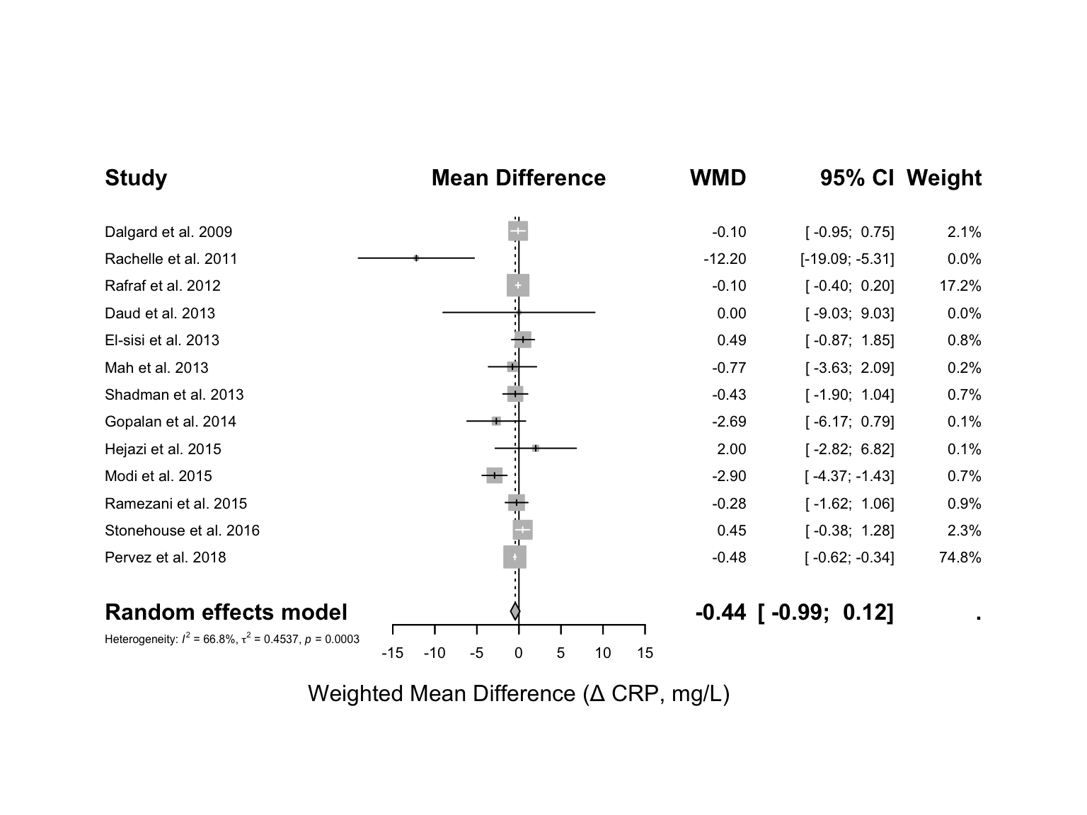
You can modify your plot using the various options offered by the forest() function. To see all available options, run ?forest in your console.

In the next part, we will explore finding the sources of heterogeneity, which will lead us to performing subgroup analyses.

Stay tuned!